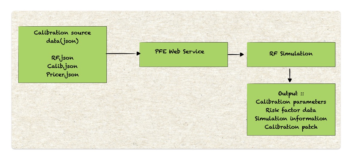
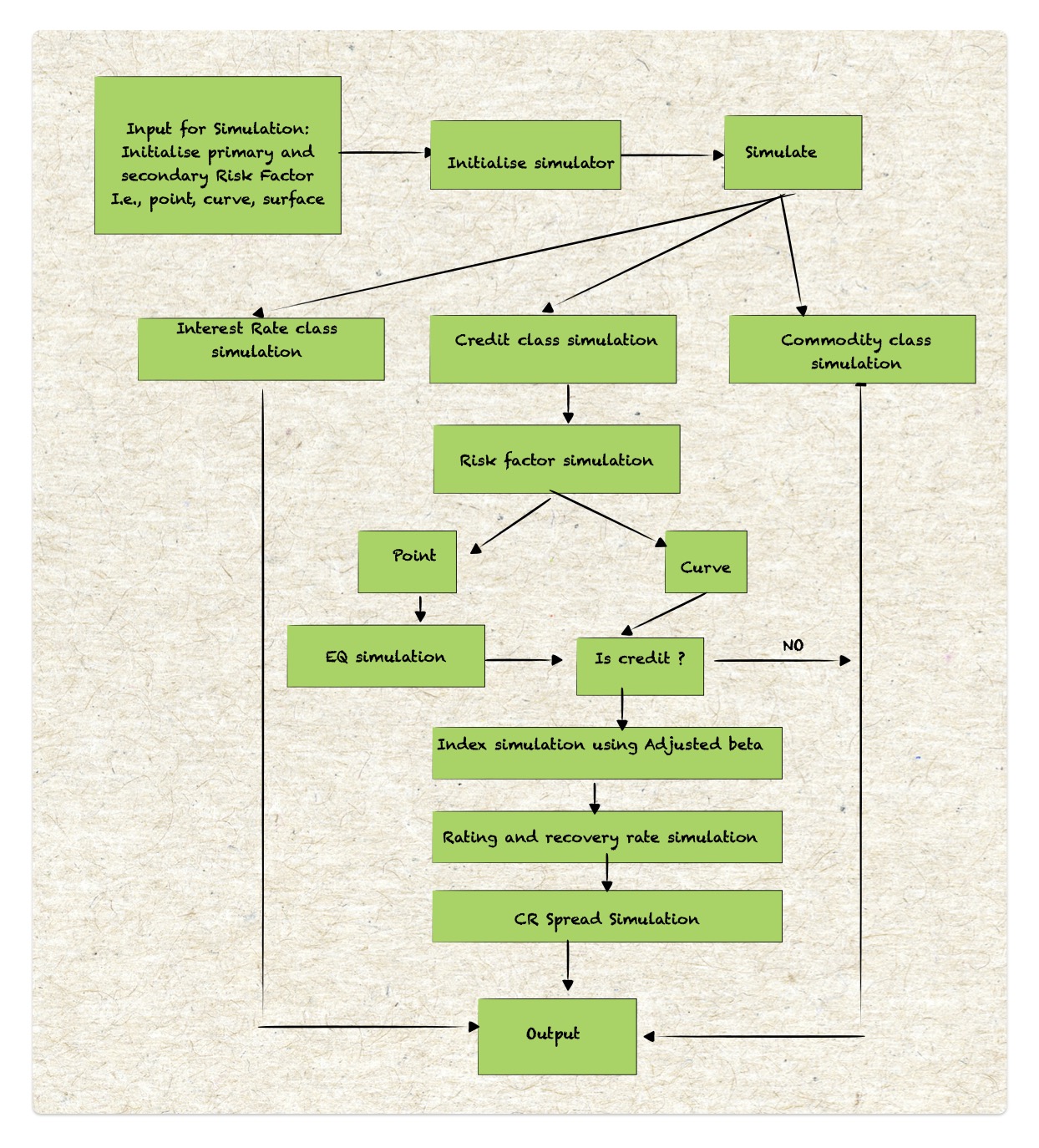
The primary goal of Potential Future Exposure (PFE) Simulation is to generate future scenarios for correlated risk factors (RF). These scenarios are fed into pricers to estimate future trade-level PFE exposure across 75 pricing horizons. The results are then passed on to aggregation, where the full PFE distribution is computed at 38 time horizons at the counterparty (C/P) level. This process also accounts for netting and collateral. Following flow chart displays the flow for backtesting of exposure and risk factor simulated data.
Key steps
-
Identify primary risk factors: Select the key RFs with historical data for the trades. For example, in interest rate options, the RFs are discount rate curves, forecast curves, and rate volatilities.
- Primary vs. Secondary Risk Factors:
- Primary risk factors: Use correlated random numbers as input and leverage Front office (FO) desk models for valuation.
- Secondary risk factors: Employ approximations where necessary.
-
Simulate stochastic process: Choose reasonable dynamics to simulate stochastic processes. For example: rates curve follows a vasicek process rate volatility follows exponential vasicek.
- Model Calibration: Calibrate the models with proper correlation among RFs. Example: When market conditions suggested that interest rates could turn negative the rate curve dynamics was adjusted to the exponential vasicek model.
Pre-simulation steps
Data Collection: Gather all necessary data for RF Simulation. This includes calibration data and market data, fetched from respective databases.
Risk Factor modelling choices
a. Interest Rate (IR) Simulation:
-
Simple model: 1 factor Hull-White model.
Advantages:
Markovian (no memory)
Closed form solutions of discount factors, cap, floor and swaption pricing. - Advanced Model : SABR model which is complex but can calibrate to the entire volatility surface, including skew.
- Other options:
Gaussian one factor model : G1++
Gaussian two factor model: G2++
Quadratic Gaussian Model
b. FX Simulation:
Geometric brownian motion(GBM)
Local Volatility/ stochastic volatility models
c. Commodity RF simulation: RFs are categorised as primary and secondary. The secondary RFs are a linear transformation of the primary RFs. Perform PCA to identify key RFs, as commodities typically rely on PCA to capture the At-the-Money(ATM) volatility term structure. A shifted log-normal model is used to capture the vol-term structure, calibrated to ATM.
d. Equity Simulation: GBM with local volatility. Shifted log-normal model is the simplest model to incorporate skew into equity simulation.

