Counterparty Credit Risk (CCR) refers to the risk that a counterparty in a financial transaction will default before the final settlement of the transaction’s cash flows. Given its significance, banks aim to hedge and continuously estimate CCR. Institutions have developed internal models to estimate future risk exposure, which includes simulating underlying risk factors that impact the valuation of trades over time. Therefore, it is crucial to have a backtesting framework in place for both simulation and pricing models to evaluate their performance and ensure they can be relied upon for accurate exposure computation.
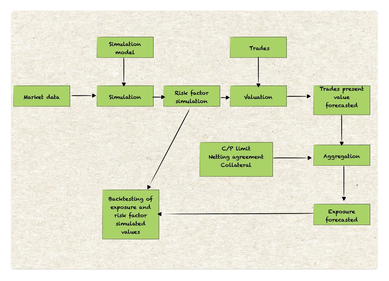
Following flow chart displays the flow for backtesting of exposure and risk factor simulated data.

This blog contains 2 parts :
Part A : Risk factor simulation backtesting
Part B : Portfolio exposure backtesting
Parameters for Backtesting
a. Testing Sample:
- In-sample test: The sampling window is the same as, or within, the calibration window.
- Out-of-sample test: The sampling window is outside the calibration window.
b. Risk Horizons for Various Products:
- OTC Derivatives: Up to 1 year
- Securities Financing Transactions (SFT) (Bonds, CMBS, RMBS/TBA): Up to 3 months
- Prime Brokerage Services: 5 days
PART A : Risk factor backtesting
Risk factor backtesting is conducted to evaluate the simulation model. The objective is to demonstrate that the distributions of the simulated paths and the historically realized values are statistically same.
Different asset classes require different risk factors to be simulated:
- Interest Rate (IR): IR Rate, IR Volatility
- Foreign Exchange (FX): FX Rate, FX Volatility
- Equity: Index, Single Name
- Commodity: Commodity Price, Commodity Volatility
- Credit: Issuer Spread, Generic Curves
Null Hypothesis:
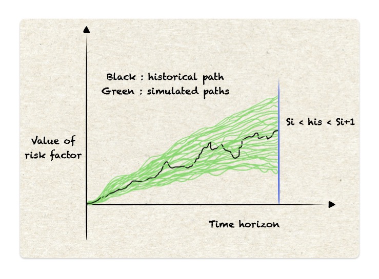
H₀: There is no statistical difference between the historical path of a risk driver and the N simulated paths.

Steps:
-
Rank the historical path among the 5000 simulated paths, i.e., $s_i$,
Rank $i$ is where $s_i < \text{his} < s_{i+1}$ -
Compute the u-value: $u = (\frac{i + (\text{his} - s_i)}{s_{i+1} - s_i} )/ N$
-
Sort the u-values and compute the distance using either the Anderson-Darling (AD) or Cramér-von Mises (CM) test.
-
Calculate the distribution distance with $U(0,1)$, denoted as $d$.
-
Obtain p-values from pre-calculated values for $d$.
Finally, combine p-values from multiple simulation re-initializations to derive a single p-value representing the overall backtesting result using Stouffer’s method of aggregation.
PART B : Portfolio exposure backtesting
Exposure backtesting is performed to evaluate pricing models.
The null hypothesis is:
H₀: The historically realized value should not show a statistical difference from the simulated exposure value. The predicted value should be greater than or equal to the realized value.
Count the sample size and the number of breaches, and test it against a Binomial distribution.
P-value = 1 - C(n,k,p)
Breaches are counted as follows: for collateralized trades, we backtest the MPoR (Margin Period of Risk) profile, and for uncollateralized trades, we test the shift profile:
a. For uncollateralized exposure: MtM > PFE profile
b. For collateralized exposure: MtM increase during MPoR > collateralized PFE profile
It is important to note that breaches can be aggregated across multiple portfolios, but not across different risk horizons.
Model performance evaluation
The final model performance is evaluated using a traffic light system based on the p-value. Green indicates healthy performance, yellow suggests the model needs attention, and red means the model is not suitable for use.
Traffic Light Criteria:
- P-value > 5%: Green
- P-value < 0.01%: Red
- Everything in between: Yellow